Somewhere off the coast of Denmark, a bright orange buoy bobs in the North Sea. It looks unremarkable – a navigation marker, maybe, or a weather float. But inside its sealed housing, a laser is firing invisible pulses of infrared light straight up into the sky, 10,000 times per second. Each pulse travels upward, scatters off microscopic dust and salt particles drifting in the wind, and returns a faint echo. By the time that echo reaches the detector, the buoy’s computer already knows the wind speed at 80 meters, at 120 meters, and at 160 meters above the ocean surface – all without a single mechanical anemometer, cable, or tall mast in sight.
The science behind this instrument is almost two centuries old. In 1842, an Austrian physicist named Christian Doppler published a paper explaining why the pitch of a sound changes when its source is moving. You hear this every time an ambulance races past you: the siren sounds higher as it approaches, then drops noticeably the moment it passes. The sound waves in front of the vehicle get compressed, raising the frequency. Behind it, they stretch out, lowering it. That shift in pitch is not a quirk of perception. It carries precise mathematical information about velocity.
Engineers discovered that the same principle works with light. Aim a laser at moving particles, measure the tiny frequency shift in the returning signal, and the wind speed is encoded right there, readable by anyone who knows the formula.
This is the Doppler effect in wind measurement. And it is quietly changing how humanity decides where to build its wind farms.
Table of Contents
Frequency Shift as a Measurement of Particle Velocity
Sound moves through air at about 343 meters per second. Light moves through space at 300,000 kilometers per second. The two seem worlds apart, yet the same frequency-shift relationship governs both – because the underlying physics is about relative motion, not about the type of wave involved.
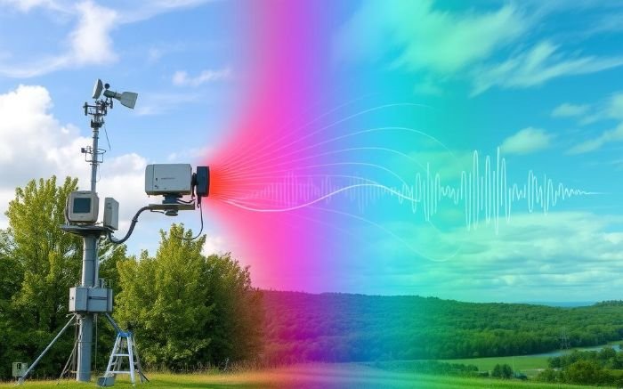
Here is how a Doppler wind measurement actually works. A transmitter fires a beam of laser light into the atmosphere. That beam strikes microscopic airborne particles: dust grains, sea salt crystals, pollen, tiny water droplets. Most of these particles are between 0.1 and 10 micrometers in diameter, smaller than a human red blood cell. Each one scatters a tiny fraction of the beam back toward the instrument. Because the particles are moving with the wind, the scattered light returns at a slightly different frequency from what was originally transmitted. The instrument measures that difference, and from it calculates the wind speed.
The formula is straightforward. If the transmitter sends a signal at frequency f₀, and particles are moving toward the sensor at velocity v, the returned signal arrives at a new frequency f:
f = f₀ × (1 + v/c)
where c is the speed of the wave. A particle moving toward you compresses the wave slightly, raising the frequency. Moving away from you, it stretches the wave, lowering it. The Doppler shift Δf is the difference between what was sent and what came back:
Δf = f – f₀ = f₀ × (v/c)
Rearranging this gives wind velocity directly from the measured shift:
v = c × (Δf / f₀)
Now put real numbers in. A typical wind lidar operates at a wavelength of 1550 nanometers, which corresponds to a frequency of roughly 193 terahertz. Wind carrying aerosol particles at 10 meters per second produces a Doppler shift of about 12.9 megahertz. As a fraction of the original frequency, that is just 0.0000067 percent – an almost impossibly small change. Yet modern optical detectors resolve it cleanly enough to distinguish wind speeds to within 0.1 meters per second, better accuracy than most mechanical anemometers deliver.
Why do the particles follow the air so faithfully? Objects with mass have inertia, and inertia resists changes in velocity. A particle significantly heavier than the surrounding air would lag behind gusts and give a distorted reading. But particles below about 10 micrometers have so little mass relative to air drag that they accelerate to match the local wind speed within milliseconds. In practice, they are the wind. Measuring their velocity is measuring the velocity of the air itself.
Key Variables and Conditions That Affect Measurement Quality
Not all air is equally cooperative. The Doppler approach depends on particles being present in the beam’s path, and particle concentration varies enormously with location, altitude, and weather.
Near the ocean surface, sea spray and salt crystals create a rich scattering environment. Over dry high-altitude desert, the air can be so clean that the return signal vanishes into detector noise. Engineers check atmospheric aerosol backscatter data before deploying instruments in unfamiliar environments. Some sites simply do not contain enough natural particles to sustain reliable measurements, and the beam returns silence.
Radial Velocity and Wind Vector Reconstruction
A single beam sees only part of the wind. It detects solely the component moving directly along the beam axis – toward the instrument or away from it. This component is called the radial velocity. A wind blowing exactly perpendicular to the beam produces no Doppler shift at all and goes completely undetected by that beam alone.
To recover the full wind vector, a lidar sweeps its beam through a cone. It fires at a fixed elevation angle, typically around 15 degrees above horizontal, while rotating through 360 degrees around the vertical axis. This pattern is called a velocity-azimuth display scan, or VAD scan. At each azimuth angle θ, the measured radial velocity vr depends on two true horizontal wind components: u (blowing west to east) and v (blowing south to north):
vr(θ) = u × cos(θ) + v × sin(θ)
As the beam sweeps through many angles, this equation gets measured repeatedly with different values of θ. Solving the resulting set of equations gives the true wind components u and v. The total horizontal wind speed U follows:
U = √(u² + v²)
A commercial wind lidar typically completes 72 azimuth positions per rotation. Each full scan takes about 60 seconds and produces a vertical wind profile from 40 meters to 250 meters altitude, with a speed and direction reading every 20 meters of height.
Pulse Duration and Vertical Resolution
Every measurement involves a trade-off with no perfect solution. Longer laser pulses carry more energy and produce stronger return signals, but they smear the measurement over a larger vertical range. A 400-nanosecond pulse travels 120 meters through the atmosphere while it is transmitting, so the return signal represents an average over a 60-meter vertical layer. A 200-nanosecond pulse cuts that layer to 30 meters but with weaker signal and more noise. Most commercial wind energy lidars are tuned to deliver 20-meter range gates – each reported wind speed representing a 20-meter vertical slice of atmosphere.

Physical Limits of Doppler Wind Measurement
Physics sets hard ceilings on what any Doppler system can achieve. The first is called the Nyquist velocity limit, and it comes from the way pulsed instruments work.
A pulsed lidar does not transmit continuously. It fires short bursts and listens between them. The rate at which it fires is called the pulse repetition frequency, or PRF. If the wind is moving fast enough, the phase of the returning signal shifts by more than half a cycle between pulses, and the instrument misreads this as a slower wind blowing in the opposite direction. The maximum unambiguous wind speed is:
v_max = λ × PRF / 4
A lidar operating at 1550 nm wavelength with a PRF of 20 kilohertz hits this ceiling at about 7.75 meters per second – far too low for wind energy applications. Engineers solve this by transmitting alternately at two different PRF values and combining the results. This dual-PRF technique extends the usable measurement range above 30 meters per second, covering nearly all wind speeds of commercial interest.
The second limit is signal-to-noise ratio. Below roughly -25 dB carrier-to-noise ratio, the weak return from distant aerosol particles drowns in detector noise. In very clean air – over the central Pacific, or high above the Sahara – this threshold cannot be reached and the measurement simply fails. Data gaps in lidar records often trace back to temporarily clean air layers rather than instrument malfunction.
Rain is the third complication. Large raindrops fall at 1 to 9 meters per second, and they scatter laser light far more powerfully than aerosol particles. During heavy rain, drop fall speed creates a strong downward Doppler signal that contaminates the horizontal wind measurement. Radar-based Doppler systems handle precipitation better because centimeter-wavelength radio waves penetrate rain without the same signal corruption.
| System Type | Wavelength | Useful Range | Aerosol Sensitivity | Behavior in Rain |
|---|---|---|---|---|
| Coherent wind lidar | 1550 nm | 40-300 m | Very high | Attenuates in heavy rain |
| Doppler radar (C-band) | 5 cm | Up to 300 km | Very low | Performs well |
| Sodar (acoustic Doppler) | 3-10 kHz sound | 40-500 m | Medium | Moderate noise issues |
| UV research lidar | 355 nm | Up to 10 km | Medium | Beam blocked by heavy rain |
Everything here is free. Readers are the reason it stays that way.
I make all of it alone, with no ads. If it is worth a coffee a month to you, that keeps the next one coming.
Keep it alive →How Engineers Use Doppler Lidar for Wind Farm Site Assessment
Stand at a potential wind farm site in Portugal, looking across open rolling hillside. The terrain is rugged, permits are complex, and the nearest grid connection is 18 kilometers away. Before anyone invests a euro in construction, someone must answer a precise question: exactly how fast does the wind blow here, at what height, and for how many hours per year?
The answer to that question is worth serious money. Every 1 meter per second error in the estimated mean annual wind speed at hub height typically translates to a 5 to 8 percent error in predicted annual energy production. On a 200-megawatt project, a 6 percent error in revenue projection can shift the entire business case from profitable to unfinanceable. Banks lending to wind farm projects require energy yield assessments of bankable quality, and that means verified measurement data with documented uncertainty.
Doppler lidar entered commercial wind energy assessment around 2008 to 2010. Its arrival changed the economics of measurement campaigns significantly. Installing a 100-meter lattice tower with calibrated cup anemometers typically costs between $250,000 and $400,000. It requires permits, civil works, aviation warning lights, and months of lead time. A portable ground-based lidar unit at comparable capital cost can be unpacked from a trailer, leveled on a concrete pad, and running within a day. When the campaign ends, it loads back onto the trailer and drives to the next site.
How do engineers confirm that lidar data is accurate enough for these high-stakes decisions? The standard validation approach places a lidar directly beside an instrumented meteorological mast for three to six months. Simultaneous readings at matching heights are compared statistically. High-quality instruments consistently achieve R² correlation coefficients above 0.99 against calibrated cup anemometers. The IEC 61400-12 standard governing wind turbine power performance testing was updated to formally accept lidar measurements as a valid alternative to mast-mounted instruments.
Floating Lidar and the Offshore Wind Challenge
Installing a measurement mast in 30 meters of water costs between $5 million and $10 million. In water deeper than 50 meters, fixed masts become structurally impractical. Offshore wind development in the North Sea and along the US East Coast pushed engineers toward a different solution.
A floating lidar is a Doppler wind profiler mounted on a moored buoy. It works – but with a complication. When the buoy pitches and rolls with ocean swell, the beam tilts away from vertical. A seemingly small 2-degree tilt during a scan at 15 degrees elevation angle can introduce a 5 to 8 percent error in retrieved horizontal wind speed if left uncorrected. Over a full year of measurements, that systematic bias would completely undermine the investment decision.
Modern floating lidar systems carry inertial measurement units – the same type of sensor that tells a smartphone which way is up. These units record the buoy’s angular orientation more than 100 times per second. Motion compensation algorithms rotate each measured velocity vector back into the earth-fixed reference frame using the recorded tilt at the exact moment of each measurement. With this correction applied, floating lidar uncertainty falls within the limits acceptable for bankable energy assessments, and the $5 million fixed mast disappears from the project budget.
Open Problems: Complex Terrain and Turbulence Measurement
The VAD scan reconstruction works cleanly when the wind field is spatially uniform across the full scan cone. Over flat terrain, this assumption is reasonable. Over the rugged landscapes where wind energy developers most often want to build, it is frequently wrong.
The lidar scan cone at 100 meters altitude covers a circle roughly 200 to 400 meters in radius on the ground, depending on elevation angle. If a ridge runs across one side of that circle, air accelerates over it. If a valley sits on the other side, flow decelerates. The scan samples these different conditions simultaneously and averages them into a single wind vector that accurately represents none of them. Researchers are developing sector-scan strategies that restrict azimuth sampling to a narrow angular range aligned with the dominant wind direction, reducing the influence of terrain-driven spatial heterogeneity.
Turbulence intensity is a separate and equally stubborn problem. Turbulence describes the rapid, chaotic velocity fluctuations superimposed on the mean wind. A turbine blade encountering a sudden gust carries far higher structural loads than one moving through smooth flow. Blade fatigue life depends critically on turbulence intensity, and lenders ask for it explicitly in energy yield reports.
A lidar pulse averages wind velocity across its entire pulse volume, spanning 20 to 60 meters vertically and several meters in beam width. Turbulent eddies smaller than the pulse volume get averaged away before reaching the detector. Comparative studies consistently show that lidar systems underestimate turbulence intensity by 15 to 30 percent compared to sonic anemometers measuring at a single fixed point. Researchers are now analyzing the spectral width of the Doppler return signal rather than just its peak frequency. A broader spectral peak indicates more velocity spread within the pulse volume, which is essentially turbulence in disguise. This technique is recovering some of what averaging erases, though it has not yet reached the accuracy of direct point measurements.
Wake Mapping, Predictive Control, and Satellites
Wind energy is scaling fast. The largest offshore turbines now have rotor diameters exceeding 200 meters – blades longer than two football fields – with hub heights above 150 meters. The wind profile across that rotor disk can vary by several meters per second from tip to tip, and the turbine’s control system needs to know what it is walking into. This vertical variation in wind speed with height is known as the wind shear profile.
Networks of scanning Doppler lidars are already deployed inside operating wind farms to map wake flows in real time. When a row of turbines extracts energy from the wind, it leaves a slow-moving, turbulent wake that can stretch 5 to 10 rotor diameters downstream – more than a kilometer for the largest machines. The next row of turbines sits inside this wake and produces significantly less power. By tracking wakes with lidar, farm control systems can adjust individual turbine yaw angles to steer wakes away from downwind machines, recovering 1 to 2 percent of total farm energy output. On a 500-megawatt farm, that recovery is worth millions of dollars per year.
Predictive control goes further still. A lidar positioned 500 to 800 meters upwind of a turbine can detect an incoming gust 30 to 60 seconds before it reaches the rotor. The blade pitch control system uses that advance warning to adjust the angle of attack before the load arrives, reducing peak structural stress. Early field trials at offshore sites in the UK showed measurable reductions in blade fatigue loads, which translate directly into longer operational lifetimes and lower maintenance costs.
The widest application of Doppler wind measurement is not on land or sea at all. ESA’s Aeolus satellite, launched in 2018 and operational until 2023, carried an ultraviolet Doppler lidar at 355 nm wavelength. It fired pulses downward through the atmosphere from orbit, measuring wind profiles across the full depth of the troposphere over oceans, deserts, and mountain ranges where no ground station reaches. Incorporating Aeolus data into global weather forecast models improved prediction accuracy by 2 to 4 percent in data-sparse regions. Over the vast stretches of the Southern Ocean and central Africa, that represented genuinely new wind information entering the forecast system for the first time.
A successor constellation of such satellites could provide global wind profiles at 2-kilometer horizontal resolution, updated continuously. For wind energy developers, that would transform site prospecting. A location in the Philippines, off the coast of Morocco, or in the Patagonian steppe could be assessed from orbit before a single engineer boards a flight. The Doppler frequency shift that Christian Doppler described while listening to musicians playing on a moving railway train in 1842 has traveled a long way since then.
You read the whole thing.
That is rarer than it should be, and it is the exact kind of attention I built this archive for. I make every piece alone, with no ads and no investor deciding what gets written. If you want the next machine taken apart like this one, you can help me make it.
A coffee a month is enough to keep it free for everyone.
Prefer crypto or a one time gift? Other ways to give →
Technologies Related to This Concept
| Technology | Concept |
|---|---|
| Nano Wind Turbines Embedded in Building Facades | Tiny turbines integrated into the sides of buildings to capture wind energy. |
| Compact Bridge Wind Tunnels | Small tunnels added to bridge designs that funnel wind to internal turbines. |
| Wind-Powered Helical Wind Funnels | Compact helical structures that funnel wind to drive internal generators. |
| Ultrasonic Wind Energy Harvesters | Devices that convert wind-induced ultrasonic vibrations into electricity. |
| Dynamic Facade Panels for Wind Energy Harvesting | Facade panels that move dynamically with the wind, capturing energy through kinetic motion. |
| Energy-Producing Paints for Wind Turbine Blades | Coating wind turbine blades with solar paints to generate additional energy. |