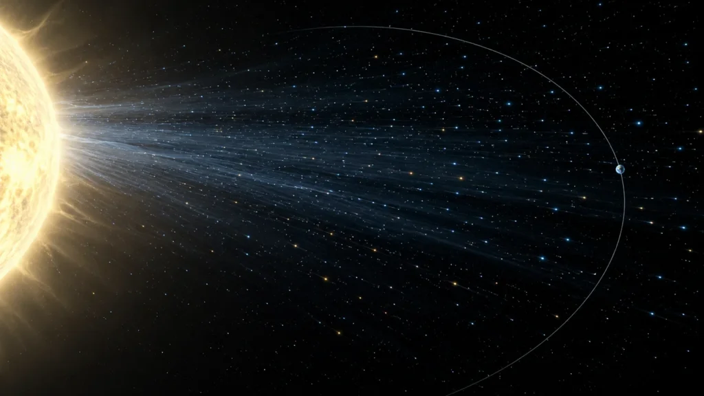
In the seventy years since the first object left Earth’s atmosphere, every spacecraft humanity has operated in heliocentric space has been flying through the same continuous particle stream without stopping to collect any of it. The solar wind at 1 AU delivers approximately 3.4 trillion charged particles through every square meter per second at an average velocity of 450 kilometers per second. The kinetic energy in that stream is real, measurable, and in a vacuum entirely conserved. A satellite designed to intercept that stream and convert what it carries into stored propellant does not exist yet. The physics for why one would work does.
The short version: Solar wind particle fuel collectors are orbital satellites equipped with superconducting magnetic scoops that concentrate and capture the continuous plasma stream the Sun emits. Protons collected at scale can be compressed into hydrogen propellant or fuel-cell feedstock. At 1 AU, solar wind carries roughly 0.57 milliwatts of kinetic energy per square meter – about 2.4 million times less than sunlight – but a magnetic field extending 500 kilometers replaces physical collection area entirely and shifts the output calculation to approximately 89 megawatts continuous. The device makes the most immediate sense as a deep-space propellant depot. What it becomes at larger scale is a different infrastructure problem.
Key Takeaways
- The scoop in a solar wind collector is not a physical surface but a magnetic field extending hundreds of kilometers – the satellite can be compact while the funnel is continental in scale
- Solar wind kinetic energy at 1 AU is 2.4 million times less dense than sunlight at the same distance, and the entire engineering argument for this device rests on a single field-geometry insight that recovers that disparity
- Helium-3 constitutes roughly 0.002% of solar wind particles but a collector operating continuously near Earth’s orbit accumulates several kilograms per year – enough to matter if fusion technology ever reaches deuterium-helium-3 operation
- A coronal mass ejection temporarily spikes particle density 50 to 100 times above baseline for hours at a time, transforming the collector’s yield without requiring any hardware change
- The long trajectory of this device class ends with autonomous refueling depots distributed through the inner heliosphere – infrastructure that removes the need to lift propellant out of Earth’s gravity well for every deep-space mission
Table of Contents
What the Solar Wind Actually Carries at 1 AU: Composition, Speed, and the Flux That Gets Ignored
There is something slightly absurd about a species that has placed dozens of instruments in heliocentric orbit to measure the solar wind in precise detail, and zero devices designed to collect from it. Every major space agency has solar wind composition data going back decades. The particles are well-characterized. The flux is known to four significant figures. Nobody has built the collector.
What the Stream Is Made Of
The breakdown at 1 AU is consistent. Roughly 95% of solar wind particles by count are protons – hydrogen nuclei stripped of their electrons. Alpha particles, helium nuclei carrying two protons and two neutrons, make up approximately 4%. Heavy ions, oxygen, carbon, and iron among them, account for less than 1% combined. Electrons run through the stream in numbers that maintain overall charge neutrality, but their mass is negligible relative to the nucleons.
Within that alpha fraction sits something worth identifying separately: helium-3. The ratio of helium-3 to helium-4 in the solar wind sits at roughly 4 parts per 10,000 in the alpha fraction, which puts helium-3 at approximately 0.002% of all solar wind particles at 1 AU. That sounds like nothing. In terms of a quantum physics-based fusion reaction running on deuterium-helium-3 cycles, which consumes grams per cycle rather than tons, a steady multi-kilogram-per-year supply from a continuously operating collector is a supply line worth designing around.
The Flux Numbers and What They Mean
Taking mid-range conditions at 1 AU – particle density around 7.5 million particles per cubic meter and average velocity of 450 kilometers per second – the particle flux through any stationary cross-sectional area follows from:
F = n × v
Where F is particles per square meter per second, n is the number density in particles per cubic meter, and v is velocity in meters per second.
F = 7.5 × 10⁶ × 4.5 × 10⁵ = 3.4 × 10¹² particles/m²/s
That is 3.4 trillion particles. A physical plate one meter square intercepts all of them geometrically. It stops almost none of them, because solar wind protons at 450 km/s pass through ordinary matter with minimal interaction. Stopping them requires either a strong magnetic field or a significant electrostatic potential – neither of which has a surface area limit the way a physical collector does. That observation is where the device starts.
How a Solar Wind Particle Collector Would Actually Work: The Magnetic Funnel and Its Electrostatic Stage
The design of a solar wind particle collector is fundamentally an argument about geometry. Getting enough particles into a useful stream requires an effective collection area orders of magnitude larger than any physical structure a rocket can deliver to orbit. The resolution to that constraint is to stop thinking about the collector as something with walls and start thinking about it as something with a field.
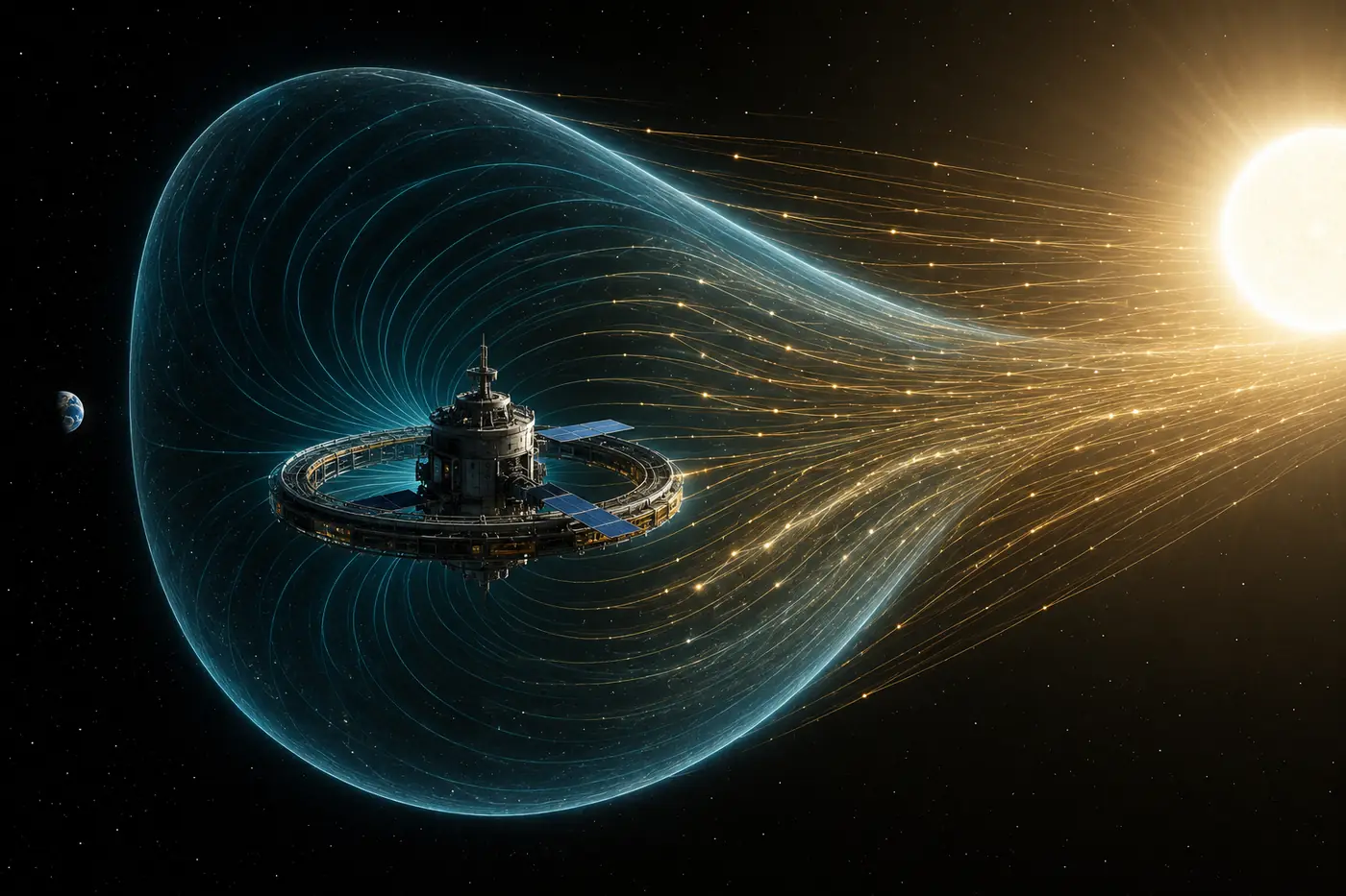
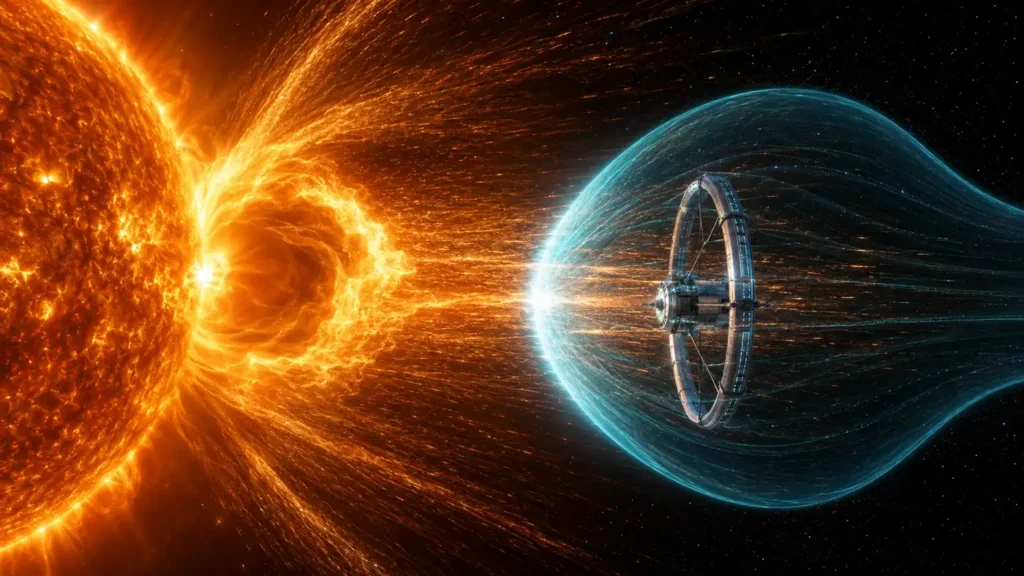
Magnetic Scoop: When the Field Becomes the Funnel
A superconducting ring carrying a large current generates a magnetic dipole field that, in the absence of atmosphere, extends outward for hundreds of kilometers. Charged particles moving through this field follow curved paths governed by the Lorentz force – the combined effect of the particle’s velocity and charge interacting with the local magnetic field strength. Particles approaching along the field’s polar axis are funneled inward toward the ring. Particles approaching from other angles are deflected along curved trajectories that, depending on field geometry, redirect them inward as well.
The effective collection radius of this setup has nothing to do with the physical dimensions of the ring itself. It is determined by how far the magnetic field extends before it becomes too weak to meaningfully deflect a proton moving at 450 km/s. For a superconducting coil generating a field strength consistent with what has been demonstrated at laboratory scale and projected to orbital infrastructure size, that radius reaches several hundred kilometers. The satellite carrying the coil might be twenty meters across. The mouth of its magnetic funnel covers an area equivalent to a small continent.
The limitation is selectivity. A magnetic field deflects charged particles without distinguishing between a proton and an alpha particle. Helium-3 and helium-4, both doubly ionized, respond nearly identically to a given field at equal velocities. A pure magnetic scoop collects everything the field intercepts – acceptable for bulk proton collection, impractical for helium-3 separation.
Electrostatic Stage: How Helium-3 Actually Gets Separated
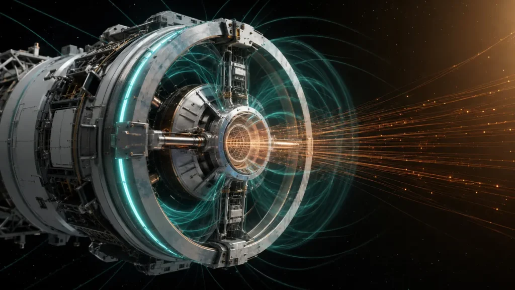
An electrostatic grid applies a strong voltage potential that attracts or repels particles according to charge and – through precise tuning of mass-to-charge ratios and particle velocities – can discriminate between species. In a full collector design, the electrostatic stage does not operate as the primary collection surface. It operates as a secondary filter at the throat of the magnetic funnel. The large magnetic field concentrates the stream. A compact high-voltage grid near the collector module’s core sorts the incoming flux.
For helium-3 separation, the device combines the spatial reach of the magnetic approach with the species selectivity of the electrostatic one. The hardware at the satellite’s core stays compact. The effective collection area is determined by the magnetic bubble, not by the grid’s physical dimensions. What the electrostatic stage adds is the ability to route the helium-3 fraction into a separate pressurized storage compartment, while the dominant proton stream feeds the hydrogen compression stage.
The Arithmetic of Dilution: 2.4 Million to One, and How a Magnetic Bubble Fixes the Scale Problem
The most important number in any solar wind collection architecture is not the flux count. It is the comparison between what the solar wind delivers per square meter and what sunlight delivers at the same distance. That comparison tells you immediately what scale of device is physically justified – and whether the argument has a shape worth pursuing.
Solar Wind Power Density vs. Solar Photon Irradiance
Each proton in the solar wind carries kinetic energy determined by its mass and velocity:
KE = ½ × m × v²
With proton mass m = 1.67 × 10⁻²⁷ kg and velocity v = 4.5 × 10⁵ m/s:
KE = ½ × 1.67 × 10⁻²⁷ × (4.5 × 10⁵)² = 1.69 × 10⁻¹⁶ J per proton
Multiplied by the flux of 3.4 × 10¹² protons per square meter per second:
P = 3.4 × 10¹² × 1.69 × 10⁻¹⁶ ≈ 5.75 × 10⁻⁴ W/m² (approximately 0.57 milliwatts per square meter)
Solar photon irradiance at 1 AU: 1,361 W/m²
The ratio: 1,361 / 0.00057 ≈ 2.4 million
Sunlight carries 2.4 million times more energy per square meter than the solar wind at the same distance. A solar panel and a proton collector placed side by side, each with a one-square-meter cross-section, are not comparable devices. Anyone framing solar wind collection as an alternative to photovoltaic collection at 1 AU has not run this number.
What a 500-Kilometer Magnetic Bubble Changes
The magnetic scoop changes the terms of the comparison by operating at a spatial scale no photovoltaic array could match. A superconducting ring achieving a magnetic capture radius of 500 kilometers presents an effective collection cross-section of:
Area = π × (500,000 m)² ≈ 7.85 × 10¹¹ m² (roughly 785,000 square kilometers)
At 0.57 mW/m², the total intercepted kinetic power from that area: approximately 447 megawatts
At a conservative 20% collection and conversion efficiency:
Continuous output ≈ 89 megawatts
89 megawatts, continuous, from a device with no combustion and no propellant supply chain attached to any planet. The gap between solar wind and sunlight per square meter disappears when the effective area jumps from 1 square meter to 785,000 square kilometers.
| Collection Method | Effective Radius | Effective Area | Continuous Power (20% eff.) |
|---|---|---|---|
| Passive physical plate | 1 m | 3 m² | 0.34 microwatts |
| Electrostatic grid alone | ~10 m | ~314 m² | ~36 microwatts |
| Small magnetic scoop | 50 km | ~7,850 km² | ~0.9 MW |
| Large magnetic scoop | 500 km | ~785,000 km² | ~89 MW |
The table has one message: physical size contributes almost nothing. Field radius is everything.
That 89-megawatt figure from a magnetic field the diameter of a small country is the number this archive was built to find.
I make all of it alone, with no ads. If it is worth a coffee a month to you, that keeps the next one coming.
Keep it alive →Positioning a Solar Wind Collector: L1, the Magnetosphere Problem, and What Inner Orbits Offer
Solar wind density does not stay constant through the heliosphere. Moving a collector closer to the Sun increases particle density and velocity, raising the kinetic power density available per square meter. At 0.5 AU, approximately Mercury’s orbital distance, particle density runs about four times higher than at 1 AU and average velocities increase. The resulting kinetic energy flux reaches 8 to 10 milliwatts per square meter – roughly 15 to 17 times higher than the Earth-orbital baseline. The arithmetic for a 500-kilometer scoop at 0.5 AU returns not 89 megawatts but something approaching 1.3 to 1.5 gigawatts at the same 20% efficiency.
The L1 Lagrange point, roughly 1.5 million kilometers sunward from Earth, offers a different kind of advantage. At L1, the gravitational balance between Earth and Sun creates a near-stable orbital position requiring minimal active maintenance. More critically, L1 sits outside Earth’s magnetosphere. A collector in low Earth orbit would find its magnetic scoop operating in direct interference with Earth’s own field, which deflects and redirects solar wind before it reaches the near-Earth environment. A collector at L1 intercepts the solar wind before the magnetosphere touches it.
Moving to 0.5 AU or closer compounds the thermal management problem sharply. The superconducting ring generating the collection field must stay below the critical temperature for its material – below 77 K for high-temperature superconductors, and ideally much colder for maximum performance. At 0.5 AU, solar irradiance reaches 5,400 watts per square meter. Maintaining cryogenic temperatures against that flux requires active radiative cooling with its own mass and power budget. The yield-versus-thermal-cost trade-off does not favor inner orbits until the cryogenic engineering reaches a performance threshold that is moving in the right direction but is not there yet. For first-generation operation, L1 is the sensible starting position.
What CME Events and Helium-3 Do to the Collection Case
The steady-state solar wind at 1 AU is the baseline the device is designed around. During a coronal mass ejection, the environment changes fast enough that the collector temporarily operates in a different numerical regime.
A CME is a large-scale ejection of magnetized plasma from the solar corona, typically triggered by magnetic reconnection events on the Sun’s surface. A major event can push particle density at 1 AU from the baseline 5 to 10 particles per cubic centimeter up to 50 to 100 or more, while simultaneously accelerating average particle velocities toward 600 to 1,000 km/s. The kinetic energy flux during a significant CME can reach 40 to 60 milliwatts per square meter – 70 to 100 times the steady baseline. For a collector with a 500-kilometer scoop, a multi-day CME represents a temporary output in the range of several hundred megawatts, automatically captured without any adjustment to the hardware.
The structural challenge is magnetic pressure. The intensified particle stream pushes harder against the collector’s field, increasing mechanical forces on the superconducting infrastructure. A field that holds stable under baseline conditions needs additional current margins to maintain its geometry during a CME without quenching – losing superconductivity abruptly due to local heating in the coils. Designing for CME survivability is not optional. The solar cycle delivers several major events per year.
Helium-3 collection operates on a different logic: patience and continuity. Continuous operation at baseline flux across a 500-kilometer capture radius yields several kilograms of helium-3 per year through the alpha fraction alone. That rate is negligible compared to the proton bulk accumulated in the same period. But the energy stored per kilogram of helium-3 in a deuterium-helium-3 fusion reaction exceeds any other practical fuel by orders of magnitude. Slow accumulation of a material that energy-dense makes the accounting work differently than the raw kilograms suggest.
From Captured Solar Wind Protons to Propellant: The Deep Space Use Case That Makes the Device Worth Building
The straightforward path from collected protons to usable fuel runs through hydrogen compression. Protons entering the collector’s throat are slowed, combined with captured electrons to form neutral hydrogen atoms, and fed into a cryogenic compression stage. The resulting liquid hydrogen is chemical propellant for conventional rocket engines or feedstock for a hydrogen fuel cell. Neither process requires novel engineering. Liquid hydrogen storage systems with long hold times already exist for launch vehicle applications. The collection stage is the novel part. The storage and delivery side runs on established infrastructure.
Deep Space as the First Productive Application
The most direct economic argument for a solar wind particle collector does not involve transmitting energy to Earth. It involves removing the requirement that every spacecraft departing for the outer solar system carry all its propellant from Earth’s surface.
A fuel depot at L1, collecting solar wind particles continuously, accumulates liquid hydrogen over months until a transfer vehicle arrives to load it. The propellant came from the solar wind, required no mining and no planetary gravity well to escape. A spacecraft on a trajectory to Jupiter stops at the L1 depot, fills its tanks, and continues with a full propellant load rather than arriving nearly empty. The economic payoff is the reduction in launch mass from Earth. How large that payoff is depends on the cost of the depot hardware versus the value of the propellant it accumulates – but the direction of the calculation is clear once launch costs drop below a threshold that several vehicle programs are approaching.
The Thermal Problem at Higher-Yield Orbits
Moving a collector to 0.5 AU to capture higher particle densities introduces thermal management requirements that go beyond incremental improvement. At that orbital distance, solar irradiance reaches four times the 1 AU value. The superconducting coils generating the collection field operate ideally below 20 K. Maintaining 20 K against 5,400 W/m² of incoming solar radiation requires a cryocooler drawing tens of kilowatts and a radiator area large enough to reject the waste heat continuously. Every kilogram added for thermal management reduces the available mass budget for the magnetic field infrastructure. An optimized design at 0.5 AU may ultimately outperform an L1 collector by a large margin. Getting there requires cryogenic material advances that are in progress but not yet deployable at the required scale.
From One Collector to a Heliospheric Fuel Network: The Evolutionary Arc of This Device Class
The first-generation solar wind particle collector is a validation instrument. Its job is to confirm that a superconducting ring in real space, exposed to real solar wind conditions including particle bombardment, thermal cycling, and CME events, holds its magnetic field geometry within acceptable parameters over months of operation. Output at this stage is secondary. Demonstrating that the physical loop closes – particles arrive, field deflects them inward, compression stores them, hardware survives – is the milestone.
The second generation scales the magnetic field radius and adds modular storage. A cluster of collectors operating near L1 at different orbital positions begins to collectively process a fraction of the local solar wind with a combined output worth planning logistics around. Individual collectors do not need to coordinate for collection purposes – each operates independently and a transfer vehicle consolidates the accumulated propellant on a scheduled basis. The depot becomes operationally self-sustaining when its combined annual output exceeds the propellant requirements of the transfer vehicle itself.
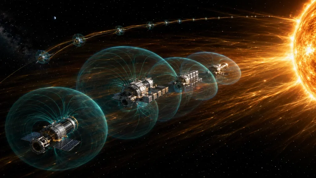
The third form belongs at the civilizational end of the arc: a distributed network of collectors positioned through the inner heliosphere between 0.5 and 1.5 AU. At that scale, the device is no longer a satellite with a purpose. It is infrastructure. Spacecraft operating anywhere in the inner solar system have access to accumulated propellant without departing from a planetary surface with a full fuel load. Lunar and Martian operations draw on a propellant supply that the solar wind replenishes continuously without being diminished by the collecting.
A device that takes without depleting, from a source that runs on the same fusion process that built every heavy element in the solar system, has a different longevity argument than any technology dependent on extracting finite reserves from a planet’s crust. The Sun has been shedding a million tons of plasma per second for four billion years. The total mass any plausible collector array could intercept in a century is unmeasurable against that outflow.
The View From NoSuchDevice
I find solar wind particle collection genuinely interesting, but probably not for the reason the concept usually gets introduced. Most descriptions of this idea lean toward its energy potential for Earth. I think that framing misses what the device is actually good for – and it misses it because the numbers at 1 AU make photovoltaic collection look more attractive per square meter by a factor of 2.4 million. Comparing a solar wind collector to a solar panel is solving the wrong problem.
The right problem is propellant, not electricity. The reason deep space missions are expensive is not primarily the hardware. It is the cost of lifting every kilogram of propellant out of Earth’s gravity well before anything can go anywhere useful. A collector at L1 that continuously accumulates liquid hydrogen from solar wind particles is not in competition with solar panels. It is a different kind of infrastructure – one that removes a mass constraint from every mission that stops there.
The helium-3 angle is slower and more speculative, but I find it more compelling over a longer horizon. The quantity accumulated per year through a 500-kilometer scoop is modest by industrial standards. The potential energy density of helium-3 in a fusion reactor is not modest by any standard. A device that accumulates a few kilograms per year of the densest practical fusion fuel identified so far, from a source that never runs low, is not a curiosity. It is a patience-based play on the future of energy technology.
What I think this device is, honestly, is a very good idea for a species that has committed to operating beyond low Earth orbit. For a species that has not made that commitment, it is a clever physics demonstration with limited near-term returns. I notice that the physics has no opinion on whether that commitment gets made.
You read the whole thing.
That is rarer than it should be. A machine that accumulates propellant from the Sun’s own exhaust without consuming anything is the kind of device I built this archive to take apart seriously. I make every piece alone, with no ads and no investor deciding what gets written. If you want the next machine taken apart like this one, you can help me make it.
A coffee a month is enough to keep it free for everyone.
Prefer crypto or a one time gift? Other ways to give →